(UCSB MATRL 204) Intro to Magnetism and Magnetic Materials#
Books used for all these notes:
Griffiths E&M 4th Ed
Griffiths QM 3rd Ed
Magnetism In Condensed Matter by Stephen Blundell
(MATRL204L1) Review of Maxwell’s equations#
This topic is aimed towards its applications in Condensed Matter. The physics involved includes Electromagnetism, Statistical Mechanics, and Quantum Mechanics. Limited Classical Mechanics is also included in terms of its formalism, such as gauge transformation, canonical momentum, and such.
Brief Review of Maxwell’s equations#
Standard Maxwell’s equations#
We start off with the four Maxwell’s equations
No magnetic monopole, then how about magnetic dipole?#
Maxwell’s equation in Dielectric Materials#
And that inside materials, the Maxwell’s equation have similar forms
Linear Response of Dielectric Materials (Griffiths E&M Ch 5&6)#
And for the linear response of dielectric materials, we have
where
\(\vec{P}\) is the charge polarization;
\(\vec{M}\) is the magnetization of the material;
\(\vec{D}\) is the electric displacement field;
\(\vec{H}\) is the auxiliary magnetic field;
with \(\mu\) denoting permeability of dielectric material and \(\varepsilon\) denoting permittivity of material.
Brief Review of Vector Potential: (Griffith E&M Ch 5)#
The vector potential \(\vec{A}\) is an analog of the potential in electrostatics. For magnetostatics, it has the form of
To find the magnetic field due to the magnetic dipole moment, we can find the \(\vec{m}\) based on the diagram and substitute the \(\vec{m}\) in Cartesian/Cylindrical coordinate to Spherical Coordinate. Refer to the diagram from Griffiths’ Figure 5.54 and the spherical coordinate unit vectors.

Fig. 14 magnetic field due to a perfect dipole along z-direction.#
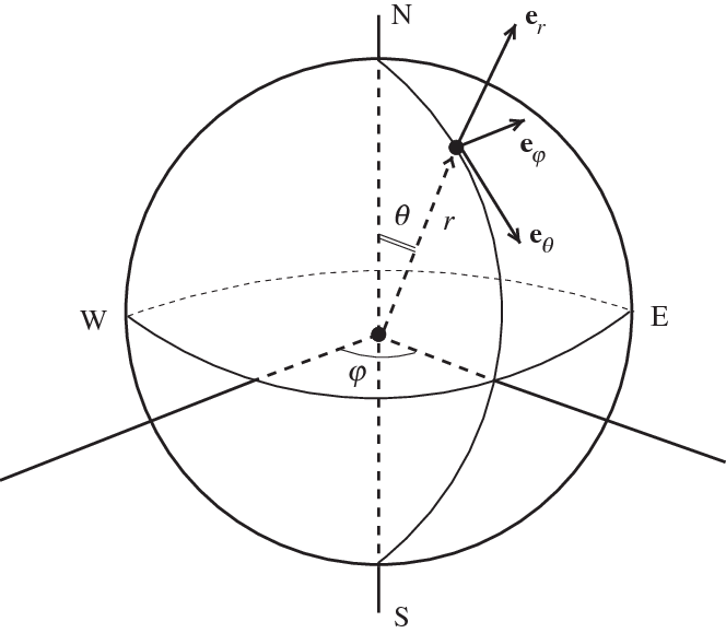
Fig. 15 Spherical Coordinate with unit vector at point (\(r\), \(\theta\),\(\phi\))#
We can then find the dot product of \(\vec{m}\) and \(\vec{r}\) and recognize that along the position vector \(\vec{r}\), \(\vec{m}\) has both \(\hat{r}\) and \(\hat{\theta}\) components, and can be found graphically. (Insert diagram of the dot product here) For this, we get
Adopting the expression that \(\vec{B}=\frac{\mu_0}{4\pi r^3}(2m\cos\theta\hat{r}+m\sin\theta\hat{\theta})\), we can simply abuse the arithmetics for a bit and get
which gives us the coordinate-free form of magnetic field expression due to a magnetic dipole moment.
Notice also that the magnetic field is partially anti-parallel to the magnetic moment, and partially parallel to the position vector along the radial direction.
Rabbit hole #001#
Alternatively, one can attempt to get lost in vector algebra, which I believe is not impossible and in fact more general, and can shed more insight into a truly coordinate-free derivation. which involves \(\nabla\times\vec{A}=\nabla\times\left[\frac{\mu_0}{4\pi}\frac{\vec{m}\times\hat{r}}{r^2}\right]\). But since we are now on a time-constraint, let’s save ourselves the mental gymnastics and pursue ideas more worthwhile, not vector and differential geometry.
Lorentz Force (Griffiths E&M Ch 10.1.4) [Needs revision]#
To briefly cover the Lorentz force, it describes when charged particles are exposed to external magnetic and electric fields. In electrodynamics, \(\nabla\times\vec{E}\) gives us a time dependent term, and can contribute to the \(\vec{A}(\vec{r}_i(t),t)\) term, affecting the magnetic field.
Recall that the convective derivative is to expose the chain rule in the partial derivative, a math trick, where (be a little more careful and revisit again)
Combining the expressions, we then yield
where \(\vec{p}_{\text{can}}=\vec{p} + q\vec{A}\) is the canonical momentum, and the \(U_{\text{vel}} = q(V-\vec{v}\cdot\vec{A})\) is the potential of velocity-dependent quantity.
Magnetization from vector and E&M standpoint:#
We have discussed in the above section that vector potential and the magnetic field are generated due to the magnetic dipole moment. But what is a dipole moment? What is magnetization?
When an electric current goes around an area \(\vec{a} = |a|\hat{n}\), a magnetic dipole moment \(\mu= Ia\hat{n}\) is generated. This is similar to but not the same description as the fourth Maxwell’s equation \(\nabla\times\vec{B}=\mu_0\vec{J}+\frac{1}{c^2}\partial_t\vec{E}\), this is different than the Amperian loop picture.
The electric current goes around like a toroid, which forms the shape of a circle. The area enclosed by a circle of radius \(r\) gives \(a=\pi r^2\) and the magnetic dipole moment is formed. The magnetic field circles around the current like a smoke vortex ring, but the dipole points upward normal to the circle. The Ampere model of magnetic dipole moment is analogous to the magnetic field in a solenoid.
Bohr-Miss van Leeuwen Theorem (brief explanation):#
Magnetization is considered a “magnetic dipole density”, or dipole moment per unit volume, induced by an external magnetic field. A brief explanation of Bohr-van Leeuwen Theorem is that a classical system does NOT have a thermal equilibruim magnetization. However, reality says you need quantum theory to address why there IS in fact a net magnetization, and so, this theorem breaks down on a quantum level.
Mathematically, we know that
So the partition function \(Z\) for N particles, and each with charge q, would take the form of
All position and momentum integrals integrate from \(-\infty\) to \(+\infty\) and that the phase space (momentum (3N) with respect to position (3N)) is \(3N + 3N = 6N\) dimensional.
Something to also keep in mind is that magnetic fields do no work because the velocity’s direction of the charged particle is perpendicular to the force produced by the \(\vec{B}\)-field. Since no work is done by the field, the energy of the system also does not explicitly depend on the external field applied. When the external \(\vec{B}\)-field is removed, then the momentum reverts, as in \(\vec{p}_{\text{can}}-q\vec{A}_i \mapsto \vec{p}_{\text{can}}\).
Questions I want to ask about lecture 1:#
Why is \(\sum\mu_s = -\mu_l\)?
The diagram shown is that the mini current curls around, we are just summing the microscopic current due to the microscopic motion of electrons, but why is the diagram showing \(\mu\) when \(\mu\) is supposed to be pointing out of page?
What exactly is this vector potential? are we taking into account that the magnetic field affects the vector potential, and not explicitly the external magnetic field, which alters the momentum of a charged particle?